Last week, I talked to a lot of students of Econometrics regarding the most difficult challenge they faced in Econometrics. The most common issue that emerged out of that discussion is constructing an econometrics model that is suitable for the data in hand and/or real world. Most often, data is not reliable as economists have to deal with secondary data which comes with many restrictions. After they get hold of data, they have to read the data, skim out the unnecessary information to fit it to the real world and economic theoretical background.
Pie-Chart shows the percentage of students facing various challenges in Econometrics.
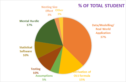
Source of the Survey: Facebook/Econometrics and Statistical Software Group
Keeping this in view, we have decided to run an article listing various types of econometrics models, one can come across. I got hold of a few, the list is not exhaustive. Our main goal is to promote the understanding of Econometrics as a subject while making the process simple and enjoyable.
What is Econometrics Modelling?
An Econometrics model is a simplified version of a real-world process, explaining complex phenomena. Behind the model, we find the application of economic theory, mathematical form, and the use of statistical tools to investigate the model.
Thus, an econometric model consists of
-
a set of equations, derived from the economic theory and mathematical model, statistical tools i.e. regression
-
Information regarding observed variables and disturbances.
-
Statement about the errors in the observed values of variables.
-
Information on the probability distribution of disturbances.
The term Econometric Modelling consists of two terms; Economic and Modelling. The econometric modeling process consists of fitting data to particular problems based on the structure of the data. Data is information, data is the new oil and to process this information, economic data should be processed in such a way that the problem can be recognized and solved.
When it comes to building a model the simplicity of the model must stand out. A model cannot be further simplified but improvement can be built upon. Look at the absolute cost advantage theory; built on a 2 sector * 2 country economy * 2 goods. What an elegant edifice on which sophisticated trade theories are based. Let’s not talk about the two sectors of the circular flow of income, Keynesian Consumption Function, and how succeeding theories were an improvement over this caricature. No models are long-lasting, but they provide a way of thought that makes a dent in the economics universe.
If you want to learn about modeling please click here.
Econometrics problems start with the problem statement derived from economic theory, which is then formulated using mathematics notation, intuitions. This mathematical model is the deterministic model in nature. When statistical tools are used it turns to a stochastic model, from which we get the required coefficients. The job of the investigator is to investigate the statistical model. Then model reliability is based on the passing of three tests – the goodness of fit, specification test, and out-of-sample prediction test. If the model does not pass through these three tests, you have to check your mathematical model formulation. This is an iterative procedure until your model passes the three tests just like chiseling out the rock to give birth to the statue. That is expected in a dynamic world from an economist to provide a much reliable, statistically valid model based on solid economic theory and experience.
Types of Econometrics Model
1. LINEAR REGRESSION MODELS
Linear Regression (LR) is the first and basic statistical tool an economics student comes across in Econometrics. It establishes a straightforward relationship between the independent and dependent variables. Dependent variable and Independent variable notation keep on changing in different circumstances; (Y or X). For example, Y can be consumption which depends on Income i.e X. Notation does not matter, as long as you are using the same intuition and logic for defining which variable is dependent or independent. Predictor/Predictand, regressor/regressand are the synonyms of the independent and dependent variables, respectively. Linear regression uses Ordinary Least Square (OLS) method. Log-lin model, lin-log model, reciprocal model are linear if the model is linear in parameters. It can be
a. Simple regression: it consists of one dependent variable and one independent variable.
For example – Consumption (C) and Income (Y)
C=+Y
b. Multiple Regression: contains more than one independent variable. If we take into account the family size (S), employment status of the head of the family (E) in our consumption-income regression then it will be multiple regression.
C=+Y+S+E
c. Multivariate Regression: if we consider our multiple dependent variables, then it will be a multivariate regression.
When our dependent variable C will be categorized as a high consumption group, low consumption group then it will turn into a multivariate regression model.
Disadvantages of the Linear Regression model:
-
One needs to be careful about outliers, heteroskedasticity, autocorrelation, and multicollinearity.
2. PANEL DATA MODELS
Panel Data Models are constructed by using both cross-sectional and Time series, thus integrating space and time. What was the Growth rate of India from 1991 to 2020 is a time series but if we consider it across states also, then it becomes panel data as it consists of space i.e. states also.
Panel data can be balanced when all cross-sectional units are observed in all periods or unbalanced when all cross-sectional units are not observed in all periods.
Estimation of panel data models can be done using the fixed effects approach, and random effects approach.
In fixed-effects approach, can have variants –
-
Intercept and slope coefficients are constant across space and time, and the error term captures the changes over time and space
-
Slope coefficients are constant but intercept changes over space or/and time
-
All coefficients are changing over space or/and time
In the Random Effects approach, the intercept is allowed to vary across time and space. This will be captured in the error components.
Associated Problems:
Besides the design and data collection problems, one has to be careful about the distortion of measurement errors, cross-section dependence, sample selectivity problems, Short time-series dimension while dealing with panel data models.
3. PROBIT AND LOGIT MODELS
When the dependent variable is a binary response, commonly coded as a 0 or 1 variable, we use Probit and Logit models.
For example, the decision/choice to whether or not a person is eligible for a loan, an individual to vote for a political party or not.
Based on the nature of choices available for the dependent variable, there can be 3 types of probit and logit model
-
Bivariate Probit and Logit Models
These models use binary dependent variables, commonly coded as a 0 or 1 variable. Two equations are estimated, representing dependent decisions.
-
Multinomial Probit and Logit Models
These models have a categorical, unordered dependent variable having alternative categories or choices out of which only one alternative can be selected. For example, a combo of financial investments one investor can undertake based on risk-taking capacity.
-
Ordered Probit and Logit Models
These have a dependent variable with ordered categories. When you fill out a consumer survey for pizza delivery satisfied, utterly bitterly satisfied, cheesily satisfied 🙂 or rate an app on Google Play, one to five scale, you are dealing with ordered models.
Associated problems:
Interpretation of coefficient is not straightforward.
4. Limited Dependent Variable Models
Sometimes we come across dependent variables with discrete and finite or continuous variables with several responses having a threshold limit. For example, the discrete choice of whether someone has a car or not can have two responses. Yes or no. How many hours someone worked on a day can have a continuous range of values from 0-24 hours.
Limited dependent variable models address two issues: censoring and truncation. Censoring is when the limit observations are in the sample and truncation is when the observations are not in the sample. Suppose you want to search for shoes in Google, then you come across the terms – shoes for women, shoes for men, shoes for school, shoes for running and walking. You use a truncated model where the common word is a shoe. When censoring, you got to censor data from your own data collection. Some of the models are the Tobit model (using censored sample), Truncated regression (using truncated sample), and Heckman model (sample selection model).
Associated Problems:
The error term is not normally distributed hence heteroscedasticity is a problem. The conventional t-test and F test are invalid. Potential for nonsensical prediction in this model.
5. Count Data Models
Count data models have a dependent variable that is counts (0, 1, 2, 3, and so on). Most of the data are concentrated on a few small discrete values. Examples include the number of children a couple has, the number of dentist visits per year a person makes, and the number of education trips per month that a school undertakes. Some of the models are;
-
Poisson model
-
Negative binomial model
-
Hurdle or two-part models
-
Zero-inflated models
Want to learn more, click here
Associated Problems:
Watch out for the skewed distribution of data.
6. Survival Analysis
Survival analysis, time-to-event analysis is applied when the data set includes subjects that are tracked until an event happens (failure) or we lose them from the sample. We are interested in how long the observation stays in the sample. Examples include how long a billionaire stays on the Forbes billionaire list, loan performance, and default, death of a patient under treatment.
Associated Problems:
Be careful of the skewness of the distribution.
Want to know more about the technique? I found the application of the method in this article amusing. You can extend it to study economic events too.
7. Spatial Econometrics
Spatial econometrics models are applied with spatial data that include geographical proximity. It can use coordinates or distances between the units also. Examples include estimating real estate prices in a neighborhood, the political behavior of the population of a certain region, establishing new branches of a bank corresponding to the economic behavior of the local population by using geo-coding software to the postal address/google map.
Associated Problems:
Watch out for Spatial error dependence in data.
Want to see an interesting application of the spatial econometrics method in political science? click here.
8. Quantile Regression
Also known as median regression this gives us a nonparametric regression as it doesn’t assume anything about the distribution of the variable. Another instance is when the distribution of dependent variables is multimodal, the OLS method doesn’t give us a proper estimator. In such cases, we use quantile regression.
It gives different effects along with the distribution of the dependent variable. The dependent variable may be continuous with no zeros or too many repeated values. For example, determining the factors affecting wages along with their distribution.
Associated Problems:
Watch out for the sample size, if it is smaller then the coefficient can be less efficient.
9. Propensity Score Matching
It attempts to estimate the effect of a treatment, policy, or other intervention by accounting for the covariates that predict receiving the treatment. Treatment evaluation is the estimation of the average effect of a program or treatment on the outcome of interest. A comparison of outcomes is made between treated and control groups. Propensity score matching is used when a group of subjects receives treatment and we’d like to compare their outcomes with the outcomes of a control group. Examples include estimating the effects of a training program on job performance or the effects of a government program targeted at helping particular schools.
Associated Problem:
Watch out for confounder imbalance i.e. increase in the bias due to matching since it does not account for dormant and unobserved confounding variables.
Want to learn more, here
10. Principal Component Analysis
Principal Component Analysis employs data reduction methods to re-express multivariate data with fewer dimensions. This method is used after conducting surveys to “uncover” the common factors or obtain fewer components to use in subsequent analysis. The reduced data set includes features of original data, causing the highest variance. The feature that causes the second-highest variance is the second important feature/component.
Original data PCA
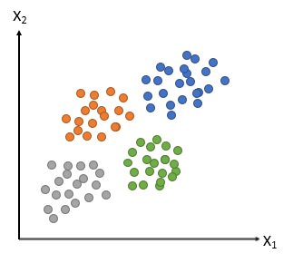
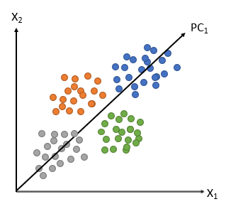
Image Source: https://bit.ly/3daiuaI
Associated problem:
Standardization of data needed. Sometimes independent variables become less interpretable.
11. Instrumental Variables Model
Instrumental variable procedures are needed when some regressors are endogenous (correlated with the error term). The procedure for correcting this endogeneity problem involves finding instruments that are correlated with the endogenous regressors but uncorrelated with the error term. Then the two-stage least squares procedure can be applied. An example of instrumental variables is when wages and education jointly depend on ability which is not directly observable, but we can use available test scores to proxy for ability.
Associated Problem:
Watch out for small sample sizes which can give biased coefficients.
12. Seemingly Unrelated Regressions Models
Seemingly unrelated regressions models invented by Gellner in 1962, uses multiple equations instead of a single equation which can be regressed and the estimator can be found independently. it is called on related seemingly because these are only related to error terms.
Example: Suppose a country has 10 states and the objective is to study the saving pattern of the country. There is one saving equation for each state. So altogether 10 equations describe 10 savings functions. It may also not be necessary that the same variables are present in all the models. Different equations may contain different variables.
13. Time Series ARIMA Models
Time series ARIMA (Auto-Regressive Integrated Moving Average) models are applied with time-series data of variables measured over time.
It has the following features:
A regressive model is a model which uses lacked dependent variable as an independent variable
Moving average model: where the mean regression back to its original one integrated when it ages nonstationary to the same degree.
The model is seated to study the present scenario and forecast the future value. Using this model you can study the relationships of variables overtime surcharge stock prices or agricultural production or effects of growth on employment or we can predict economic growth based on our past data and so on.